ifermi program
IFermi includes command-line tools for generating, analysing, and plotting Fermi
surfaces. The tools can be accessed using the ifermi command-line program.
All of the options provided in the command-line are also accessible using the
Python API.
IFermi works in 4 stages:
It loads a band structure from DFT calculation outputs.
It interpolates the band structure onto a dense k-point mesh using Fourier interpolation as implemented in BoltzTraP2.
It extracts the Fermi surface at a given energy level.
It extracts information about the Fermi surface or plots it using several plotting backends.
Note
Currently, IFermi’s command-line tools only work with VASP calculation outputs. Support for additional DFT packages will be added in a future release.
IFermi is controlled on the command-line using the ifermi command. The available
options can be listed using:
ifermi -h
Information on the Fermi surface area, dimensionality,
and orientation can be extracted using the info subcommand.
The only input required is a vasprun.xml. For example:
ifermi info
An example output for MgB2 is shown below:
Fermi Surface Summary
=====================

  # surfaces: 5
  Area: 32.745 Å⁻²

Isosurfaces
~~~~~~~~~~~

    Band    Area [Å⁻²]   Dimensionality    Orientation
  ------  ------------  ----------------  -------------
       6         1.944         2D           (0, 0, 1)
       7         4.370         1D           (0, 0, 1)
       7         2.961         2D           (0, 0, 1)
       8         3.549         1D           (0, 0, 1)
       8         3.549         1D           (0, 0, 1)
If properties are included in the Fermi surface (see Property projections), the averaged property values will also be calculated. This allows for calculation of the Fermi velocity. For example:
ifermi info --property velocity
Fermi Surface Summary
=====================

  # surfaces: 5
  Area: 32.75 Å⁻²
  Avg velocity: 9.131e+05 m/s

Isosurfaces
~~~~~~~~~~~

    Band    Area [Å⁻²]    Velocity avg [m/s]   Dimensionality    Orientation
  ------  ------------  --------------------  ----------------  -------------
       6         1.944             7.178e+05         2D           (0, 0, 1)
       7         4.370             9.092e+05      quasi-2D        (0, 0, 1)
       7         2.961             5.880e+05         2D           (0, 0, 1)
       8         3.549             1.105e+06      quasi-2D        (0, 0, 1)
       8         3.549             1.105e+06      quasi-2D        (0, 0, 1)
Fermi surfaces and slices can be visualised using the plot subcommand. Again, the
only input required is a vasprun.xml file. For example:
ifermi plot
The two subcommands info and plot share many of the same options
which we describe below.
Generation options
There are several options affect the generation of Fermi surfaces from ab initio
calculation outputs. These options are available for both the info and plot
subcommands.
Input file
IFermi will look for a vasprun.xml or vasprun.xml.gz file in the current directory.
To specify a particular vasprun file the --filename (or -f for short) option
can be used:
ifermi plot --filename my_vasprun.xml
Interpolation factor
The band structure extracted from the vasprun must be processed before the Fermi surface can be generated. The two key issues are:
It may only contain the irreducible portion of the Brillouin zone (if symmetry was used in the calculation) and therefore may not contain enough information to plot the Fermi surface across the full reciprocal lattice.
It may have been calculated on a relatively coarse k-point mesh and will therefore produce a rather jagged Fermi surface.
Both issues can be solved by interpolating the band structure onto a denser k-point mesh. This is achieved by using BoltzTraP2 to Fourier interpolate the eigenvalues onto a denser mesh that covers the full Brillouin zone.
The degree of interpolation is controlled by the --interpolation-factor (-i)
argument. A value of 8 (the default value), roughly indicates that the interpolated band
structure will contain 8x as many k-points. Increasing the interpolation factor will
result in smoother Fermi surfaces. For example:
ifermi plot --interpolation-factor 10
Warning
As the interpolation increases, the generation of the Fermi surface, analysis and plotting will take a longer time and can result in large file sizes.
Fermi surface energy
The energy level offset at which the Fermi surface is calculated is controlled by the
--mu option. The energy level is given relative to the Fermi level of the VASP
calculation and is given in eV. By default, the Fermi surface is calculated at
mu = 0, i.e., at the Fermi level.
For gapped materials, mu must be selected so that it falls within the
conduction or valence bands otherwise no Fermi surface will be obtained. For
example. The following command will generate the Fermi surface at 1 eV above the Fermi
level:
ifermi plot --mu 1
Property projections
Additional properties, such as the group velocity and orbital magnetisation (spin
texture), can be projected onto the Fermi surface using the --property option. The
group velocities are calculated during Fourier interpolation (units of m/s) and can be
included in the Fermi surface using:
ifermi plot --property velocity
For calculations performed using spin–orbit coupling or non-collinear magnetism, the spin magnetisation can be projected onto the Fermi surface using:
ifermi plot --property spin
Warning
Projecting the spin magnetisation requires the k-point mesh to cover the entire
Brillouin zone. I.e., the DFT calculation must have been performed without symmetry
(ISYM = - 1 in VASP).
It is possible to calculate the scalar projection of the the Fermi surface properties
onto a cartesian axis using the --projection-axis option.. For example, to use the
scalar projection of the spin magnetisation onto the [0 0 1] cartesian direction:
ifermi plot --property spin --projection-axis 0 0 1
Reciprocal space
By default, the Wigner–Seitz cell is used to contain to the Fermi surface. The
parallelepiped reciprocal lattice cell can be used instead by selecting the
--no-wigner option. For example:
ifermi plot --no-wigner
Visualisation options
In addition to the options for generating Fermi surfaces, there are several options
that control the visualisation parameters. These options are only available for the
plot subcommand.
Plotting backend
IFermi supports multiple plotting backends. The default is to the plotly package but matplotlib and mayavi are also supported.
Note
The mayavi dependencies are not installed by default. To use this backend, follow
the installation instructions here
and then install IFermi using pip install ifermi[mayavi].
Different plotting packages can be specified using the --type option (-t). For
example, to use matplotlib:
ifermi plot --type matplotlib
Output files
By default, IFermi generates interactive plots. To generate static images, an output
file can be specified using the --output (-o) option. For example:
ifermi plot --output fermi-surface.jpg
Note
Saving graphical output files with the plotly backend requires plotly-orca to be installed.
Running the above command in the examples/MgB2 directory produces the plot:
Interactive plots can be saved to a html file using the plotly backend by specifying a html filename. This will prevent the plot from being opened automatically.
ifermi plot --output fermi-surface.html
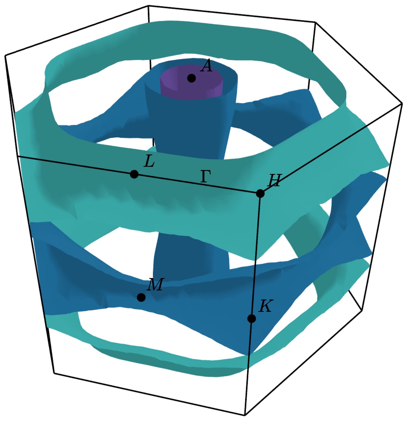
Selecting spin channels
In the plot above, the spins are degenerate (the Hamiltonian does not differentiate
between the up and down spins). This is why the surface looks dappled, IFermi
is plotting two redundant surfaces. To stop it from doing this, we can specify that
only one spin component should be plotted using the --spin option. The default
is to plot both spins but a single spin channel can be selected through the names
“up” and “down”. For example:
ifermi plot --spin up
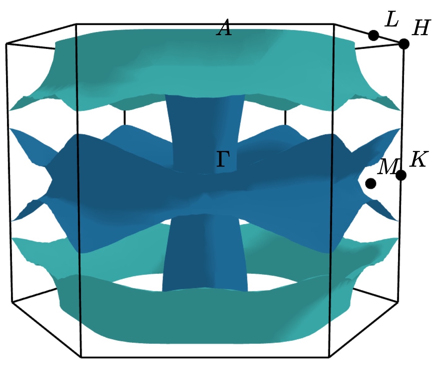
Changing the viewpoint
The viewpoint (camera angle) can be changed using the --azimuth (-a) and
--elevation (-e) options. This will change both the initial viewpoint
for interactive plots, and the final viewpoint for static plots. To summarize:
The azimuth is the angle subtended by the viewpoint position vector on a sphere projected onto the x-y plane in degrees. The default is 45°.
The elevation (or zenith) is the angle subtended by the viewpoint position vector and the z-axis. The default is 35°.
The viewpoint always directed to the center of the the Fermi surface (position [0 0 0]). As an example, the viewpoint could be changed using:
ifermi plot --azimuth 120 --elevation 5
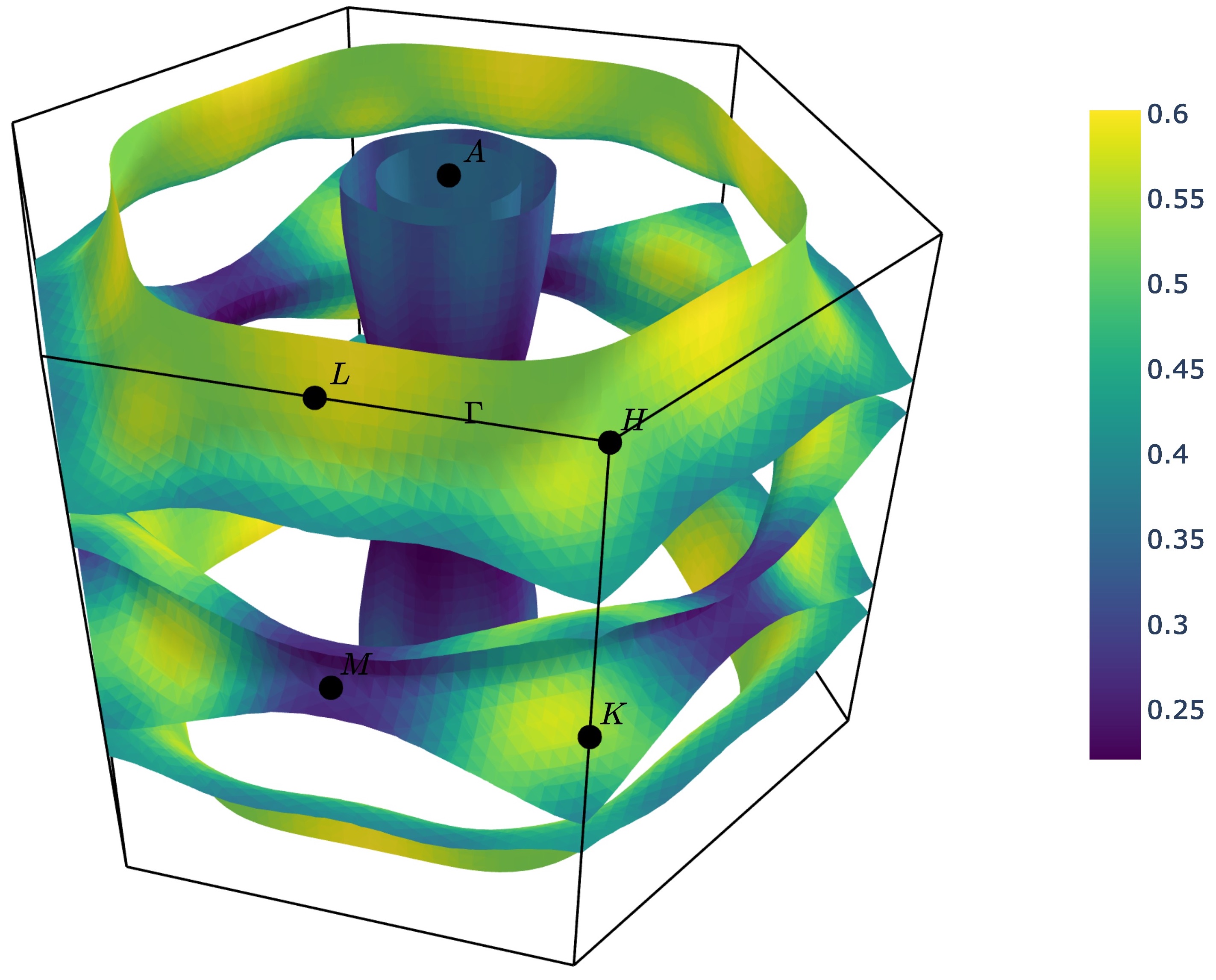
Styling face properties
As described in the Property projections section, Fermi surfaces (and Fermi slices)
can include a property projected onto the isosurface faces. By default, if properties
are included in the Fermi surface they will be indicated by coloring of the isosurface.
If the face property is a vector, the norm of the vector will be used as the
color intensity. The colormap of the surface can be changed using the
--property-colormap option. All matplotlib colormaps
are supported. For example:
ifermi plot --property velocity --property-colormap viridis
The minimum and maximum values for the colorbar limits can be set using the --cmin
and --cmax parameters. These should be used when quantitatively comparing surface
properties between two plots. For example:
ifermi plot --property velocity --cmin 0 --cmax 5
As described above, it is also possible calculate the scalar projection of the
face properties onto a cartesian axis using the --projection-axis option. When
combined with a diverging colormap this can be used to indicate surface properties that
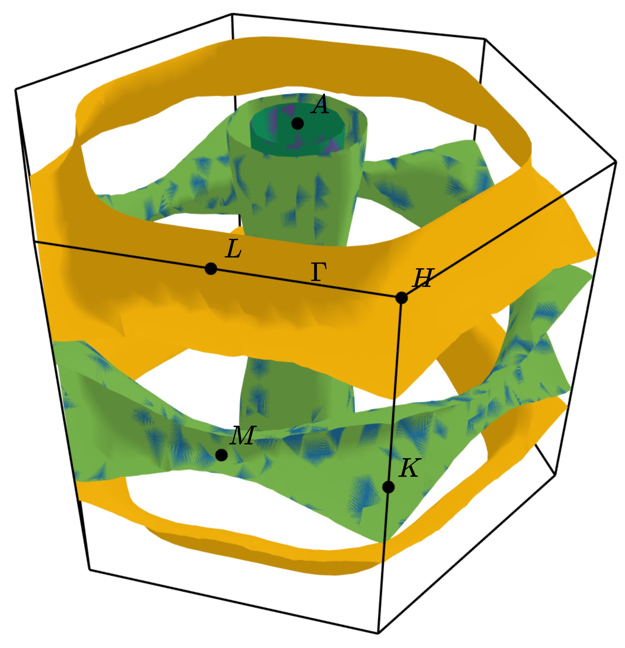
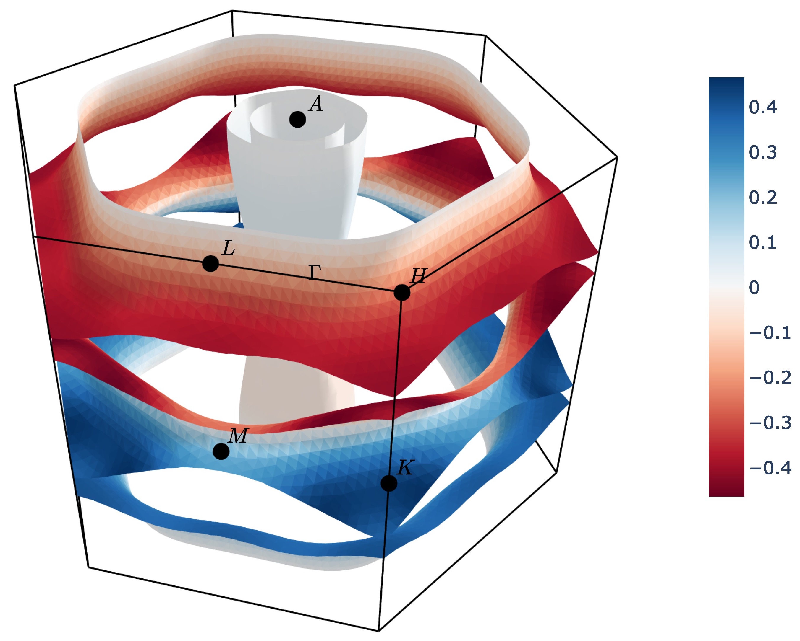
vary between positive and negative numbers. For example, below we color the Fermi
surface of MgB2 by the projection of the group velocity onto the [0 0 1] vector (z-axis).
ifermi plot --property velocity --projection-axis 0 0 1 --property-colormap RdBu
Vector valued Fermi surface properties (such as group velocity or spin
magnetisation) can also be visualised as arrows using the --vector-property option.
If --projection-axis is set, the color of the arrows will be determined by the
scalar projection of the property vectors onto the specified axis, otherwise the norm
of the projections will be used. The colormap used to color the arrows is specified
using --vector-colormap. Lastly, often it is useful to hide the isosurface
(--hide-surface option) or high-symmetry labels (-hide-labels)
when visualising arrows. An example of how to combine these options is given below:
ifermi plot --property velocity --projection-axis 0 0 1 --property-colormap RdBu \
            --vector-property --vector-colormap RdBu --hide-surface --hide-labels
The size of the arrows can be controlled using the --vnorm parameter. This is
particularly useful when quantitatively comparing vector properties across multiple
Fermi surfaces. A larger vnorm value will increase the size of the arrows.
The spacing between the arrows is controlled by the --vector-spacing option. Smaller
values will increase the density of the arrows.
Fermi slices
IFermi can also generate two-dimensional slices of the Fermi surface along a specified
plane using the --slice option. Planes are defined by their miller indices (a b c)
and a distance from the plane, d. Most of the above options also apply to to Fermi slices,
however, slices are always plotted using matplotlib as the backend.
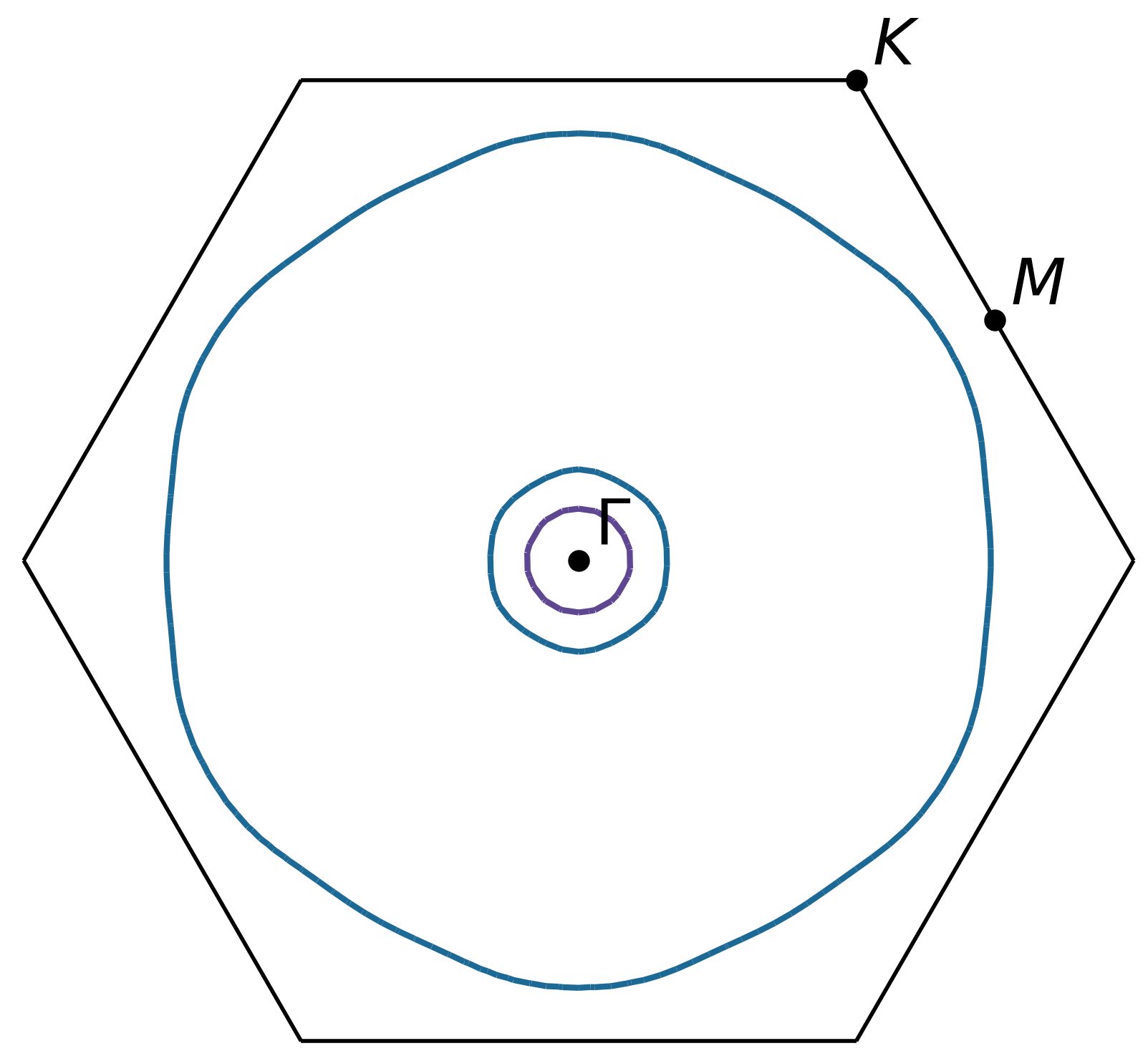
For example, a slice through the (0 0 1) plane that passes through the center of the Brillouin zone (Γ-point) can be generated using:
ifermi plot --slice 0 0 1 0
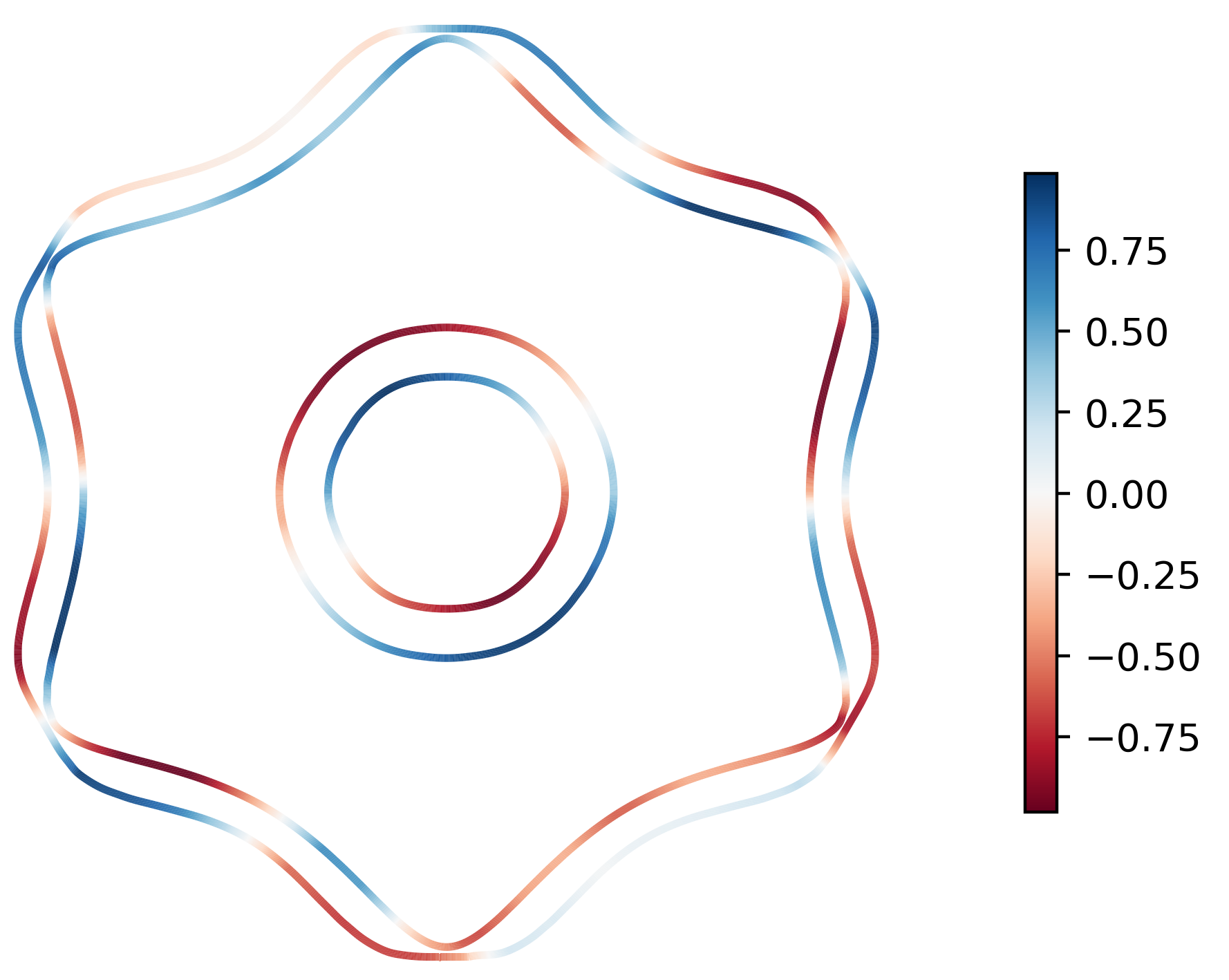
Slices can contain segment properties in the same way that surfaces can contain face
properties. To style slices with projections see Styling face properties.
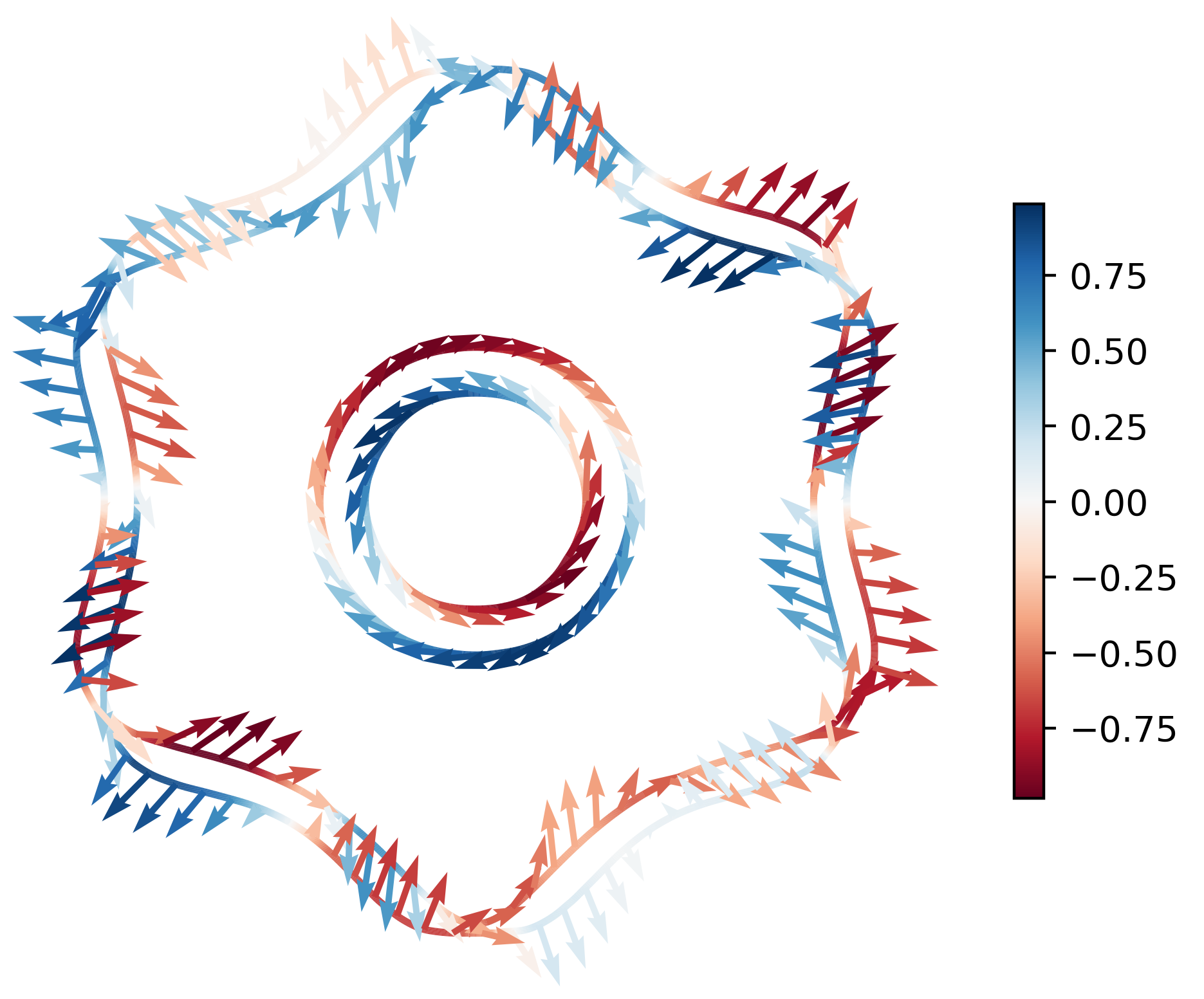
When including arrows in Fermi slice figures, only the components of the
arrows in the 2D plane will be shown. As an example below we plot the spin texture of
BiSb (examples/BiSb) with and without arrows. The spin texture is colored by the
projection of the spin onto the [0 0 1] cartesian direction.
Without arrows:
ifermi plot --mu -0.85  -i 10 --slice 0 0 1 0 --property spin --hide-cell \
            --hide-labels --projection-axis 0 1 0 --property-colormap RdBu
With arrows:
ifermi plot --mu -0.85  -i 10 --slice 0 0 1 0 --property spin --hide-cell \
            --hide-labels --projection-axis 0 1 0 --property-colormap RdBu \
            --vector-property --vector-colormap RdBu --vnorm 5 --vector-spacing 0.025
Warning
When generating spin texture plots for small regions of k-space, for example, in a small area around the Γ-point, it is often necessary to increase the k-point mesh density of the underlying DFT calculation. In the example above, the DFT calculation was performed on a 21x21x21 k-point mesh.
Furthermore, projecting the spin magnetisation requires the k-point mesh to cover
the entire Brillouin zone. I.e., the DFT calculation must have been performed
without symmetry (ISYM = - 1 in VASP).
ifermi reference
ifermi
IFermi is a tool for the generation, analysis and plotting of Fermi surfaces.
ifermi [OPTIONS] COMMAND [ARGS]...
info
Calculate information about the Fermi surface.
ifermi info [OPTIONS]
Options
- -f, --filename <filename>
vasprun.xml file to plot
- -m, --mu <mu>
offset from the Fermi level at which to calculate Fermi surface
- Default:
0.0
- --wigner, --no-wigner
use Wigner-Seitz cell rather than reciprocal lattice parallelepiped
- Default:
True
- -i, --interpolation-factor <interpolation_factor>
interpolation factor for band structure
- Default:
8.0
- --property <property>
projection type
- Options:
velocity | spin
- --projection-axis <projection_axis>
use dot product of property onto cartesian axis (e.g. 0 0 1)
- --decimate-factor <decimate_factor>
factor by which to decimate surfaces (i.e. 0.8 gives 20 % fewer faces)
- --smooth
smooth the Fermi surface
- Default:
False
- --norm, --no-norm
average property norms (overridden by –projection-axis)
- Default:
True
- --precision <precision>
number of decimal places in output
- Default:
4
plot
Plot a Fermi surface from a vasprun.xml file.
ifermi plot [OPTIONS]
Options
- -f, --filename <filename>
vasprun.xml file to plot
- -m, --mu <mu>
offset from the Fermi level at which to calculate Fermi surface
- Default:
0.0
- --wigner, --no-wigner
use Wigner-Seitz cell rather than reciprocal lattice parallelepiped
- Default:
True
- -i, --interpolation-factor <interpolation_factor>
interpolation factor for band structure
- Default:
8.0
- --property <property>
projection type
- Options:
velocity | spin
- --projection-axis <projection_axis>
use dot product of property onto cartesian axis (e.g. 0 0 1)
- --decimate-factor <decimate_factor>
factor by which to decimate surfaces (i.e. 0.8 gives 20 % fewer faces)
- --smooth
smooth the Fermi surface
- Default:
False
- -o, --output <output_filename>
output filename
- -s, --symprec <symprec>
symmetry precision in Å
- Default:
0.001
- -a, --azimuth <azimuth>
viewpoint azimuth angle in °
- Default:
45.0
- -e, --elevation <elevation>
viewpoint elevation angle in °
- Default:
35.0
- -t, --type <plot_type>
plotting type
- Default:
'plotly'- Options:
matplotlib | plotly | mayavi
- --color-property, --no-color-property
color Fermi surface properties
- Default:
True
- --property-colormap <property_colormap>
matplotlib colormap name for properties
- --vector-property, --no-vector-property
show vector properties as arrows
- Default:
False
- --vector-colormap <vector_colormap>
matplotlib colormap name for vectors
- --vector-spacing <vector_spacing>
spacing between property arrows
- Default:
0.2
- --cmin <cmin>
minimum intensity on property colorbar
- --cmax <cmax>
maximum intensity on property colorbar
- --vnorm <vnorm>
value by which to normalise vector lengths
- --scale-linewidth
scale Fermi slice thickness by property
- Default:
False
- --hide-surface
hide the Fermi surface
- Default:
False
- --plot-index <plot_index>
plot specific bands indices (1 based)
- --hide-labels
hide the high-symmetry k-point labels
- Default:
False
- --hide-cell
hide reciprocal cell boundary
- Default:
False
- --spin <spin>
select spin channel
- Options:
up | down
- --slice <slice>
slice through the Brillouin zone (format: j k l dist)
- --scale <scale>
scale for image resolution
- Default:
4